Digital filter

In electronics, computer science and mathematics, a digital filter is a system that performs mathematical operations on a sampled, discrete-time signal to reduce or enhance certain aspects of that signal. This is in contrast to the other major type of electronic filter, the analog filter, which is an electronic circuit operating on continuous-time analog signals. An analog signal may be processed by a digital filter by first being digitized and represented as a sequence of numbers, then manipulated mathematically, and then reconstructed as a new analog signal (see digital signal processing). In an analog filter, the input signal is "directly" manipulated by the circuit.
A digital filter system usually consists of an analog-to-digital converter to sample the input signal, followed by a microprocessor and some peripheral components such as memory to store data and filter coefficients etc. Finally a digital-to-analog converter to complete the output stage. Program Instructions (software) running on the microprocessor implement the digital filter by performing the necessary mathematical operations on the numbers received from the ADC. In some high performance applications, an FPGA or ASIC is used instead of a general purpose microprocessor, or a specialized DSP with specific paralleled architecture for expediting operations such as filtering.
Digital filters may be more expensive than an equivalent analog filter due to their increased complexity, but they make practical many designs that are impractical or impossible as analog filters. Since digital filters use a sampling process and discrete-time processing, they experience latency (the difference in time between the input and the response), which is almost irrelevant in analog filters.
Digital filters are commonplace and an essential element of everyday electronics such as radios, cellphones, and stereo receive

Characterization of digital filters

A digital filter is characterized by its transfer function, or equivalently, its difference equation. Mathematical analysis of the transfer function can describe how it will respond to any input. As such, designing a filter consists of developing specifications appropriate to the problem (for example, a second-order low pass filter with a specific cut-off frequency), and then producing a transfer function which meets the specifications.
The transfer function for a linear, time-invariant, digital filter can be expressed as a transfer function in the Z-domain; if it is causal, then it has the form:

where the order of the filter is the greater of N or M. See Z-transform's LCCD equation for further discussion of this transfer function.
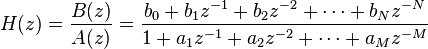
This is the form for a recursive filter with both the inputs (Numerator) and outputs (Denominator), which typically leads to an IIR infinite impulse response behaviour, but if the denominator is made equal to unity i.e. no feedback, then this becomes an FIR or finite impulse response filter.

Analysis techniques

A variety of mathematical techniques may be employed to analyze the behaviour of a given digital filter. Many of these analysis techniques may also be employed in designs, and often form the basis of a filter specification.
Typically, one analyzes filters by calculating how the filter will respond to a simple input such as an impulse response. One can then extend this information to visualize the filter's response to more complex signals. Riemann spheres have been used, together with digital video, for this purpose.

Impulse response

 

The impulse response, often denoted h[k] or h_k, is a measurement of how a filter will respond to the Kronecker delta function. For example, given a difference equation, one would set x₀ = 1 and x_k = 0 for and evaluate. The impulse response is a characterization of the filter's behaviour. Digital filters are typically considered in two categories: infinite impulse response (IIR) and finite impulse response (FIR). In the case of linear time-invariant FIR filters, the impulse response is exactly equal to the sequence of filter coefficients:

IIR filters on the other hand are recursive, with the output depending on both current and previous inputs as well as previous outputs. The general form of the an IIR filter is thus:

Plotting the impulse response will reveal how a filter will respond to a sudden, momentary disturbance.

[edit] Difference equation

In discrete-time systems, the digital filter is often implemented by converting the transfer function to a linear constant-coefficient difference equation (LCCD) via the Z-transform. The discrete frequency-domain transfer function is written as the ratio of two polynomials. For example:

This is expanded:

and divided by the highest order of z:

The coefficients of the denominator, a_k, are the 'feed-backward' coefficients and the coefficients of the numerator are the 'feed-forward' coefficients, b_k. The resultant linear difference equation is:

or, for the example above:

rearranging terms:

then by taking the inverse z-transform:

and finally, by solving for y[n]:

This equation shows how to compute the next output sample, y[n], in terms of the past outputs, y[n − p], the present input, x[n], and the past inputs, x[n − p]. Applying the filter to an input in this form is equivalent to a Direct Form I or II realization, depending on the exact order of evaluation.

Filter design

Filter design is the process of designing a filter (in the sense in which the term is used in signal processing, statistics, and applied mathematics), often a linear shift-invariant filter, which satisfies a set of requirements, some of which are contradictory. The problem is to find a realization of the filter which meets each of the requirements to a sufficient degree to make it useful.
The filter design process can be described as an optimization problem where each requirement contributes with a term to an error function which should be minimized. Certain parts of the design process can be automated, but normally an experienced electrical engineer is needed to get a good result.